"After a small Technical Pullback from $1,240 per ounce, Gold price will likely move up to test $1,500 per ounce through Dec 2016."(By a commentator to one of my articles).
The commentator is sure that the gold price is $1,500 per ounce in 2016.
Well, I will estimate the price of gold through 2016, 2017 and 2018. I will follow a traditional way to analyze time series of gold prices with an additive model. The model is formalized by a mathematical equation with 3 components.
I will use the same model from this study (Shafiee, Shahriar, and Erkan Topal. "An overview of global gold market and gold price forecasting." Resources Policy 35.3 (2010): 178-189. Source:here), but with some variations.
The model of the study in question proposes that historical data of mineral commodities have 3 terms to demonstrate a fluctuation in prices:
- a long-term trend reversion component
- a diffusion component
- and a jump or dip component.
The model calculates each term individually to estimate future prices of mineral commodities.
The study quoted validates the model and estimates the gold price for the next 10 years, based on monthly historical data of nominal gold price.
"The results indicated that, assuming the current price jump initiated in 2007 behaves in the same manner as that experienced in 1978, the gold price would stay abnormally high up to the end of 2014. After that, the price would revert to the long-term trend until 2018."(here).
I want to see if I get the same findings on updated gold prices (the study in question covers the period from January 1968 to December 2008). I will estimate 2016, 2017 and 2018 average quarterly gold prices on the ground of average quarterly gold prices from January 1968 to December 2015.
First component: Y'=alfa + beta*t' (drift in the gold price). The easiest trend is the linear one.
Y: is the time series of the gold price from January 1968 (the gold price was freed in 1967) to December 2015. Column A in the screen shot below.
Data on historical gold prices are taken from:KITCO and fromIce Benchmark Administration,Gold Fixing Price 3:00 P.M. (London time) in London Bullion Market, based in U.S. Dollars [GOLDPMGBD228NLBM], retrieved from FRED, Federal Reserve Bank of St. Louis, February 26, 2016.
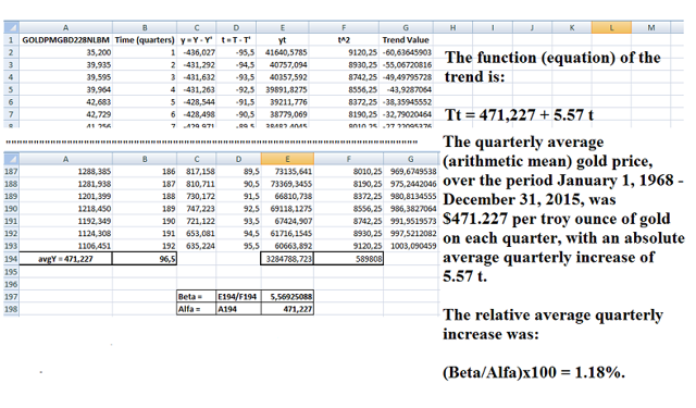
The equation of the trend of the gold price (quarterly data) over the period from January 1968 to December 2015 is:
Tt = 471.227 + 5. 57* t; where 5.57*t is the drift (first component).
Then I will replace t in the linear equation with the values of the D column (see screen shot above), to get the trend of the gold price.
Fig. 1. The quarterly historical trend of nominal gold price from January 1968 to December 2015.
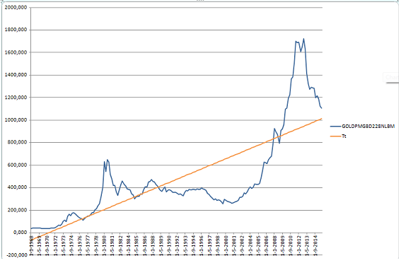
I want to point out that the trend is quite different from the function that better fits the values of the time series of the gold prices, because the trend conveys the estimated drift. In other words in order to find the trend, it is not necessary to search among different functions the one that makes the sum of the residuals the least, but the one that better conveys the drift of the phenomenon analyzed (see Girone, Giovanni, and Tommaso Salvemini. Lezioni di statistica. Cacucci, 1980).
Second component (random walk): beta*(1 + gamma), where gamma is the volatility of the gold price reverted on the trend line Tt, it has the same slope of the drift, of course.
Historical volatility or coefficient variance (gamma) is usually computed as follows:
"Historical volatility (HV) is the realized volatility of a financial instrument over a given time period. Generally, this measure is calculated by determining the average deviation from the average price of a financial instrument in the given time period. Standard deviation is the most common but not the only way to calculate historical volatility."(here).
I calculate HV in a different way (maybe the same way calculated by the authors of the study I have mentioned):
- First I calculated the residuals (Gold prices - trend values). I divided each residual by the average quarterly price of gold.
- I calculated the standard deviation of the residuals and I ran the t -test:
Then I calculate the standard error of the residuals. The standard error is none other than the standard deviation of the residuals.
"A standard error is the standard deviation of the sampling distribution of a statistic. Standard error is a statistical term that measures the accuracy with which a sample represents a population. In statistics, a sample mean deviates from the actual mean of a population; this deviation is the standard error."(here).
After I run the t-test by dividing each residual by the standard error (or the standard deviation of the sampling distribution of the residuals). I consider only those residuals which t-test is comprised between 1.96 (absolute value), at 5% confidence level. This leads me to exclude the following statistically significant AR:
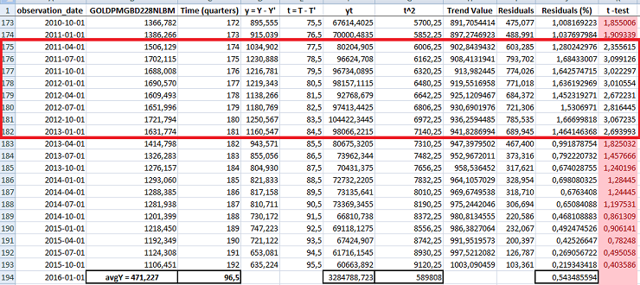
I need the residuals which are not statistically significant, that is those that fall into the 95% area of the normal (or Gaussian) distribution.
Normal distributions are important in statistics and are often used in the natural and social sciences to represent real-valued random variables whose distributions are not known.
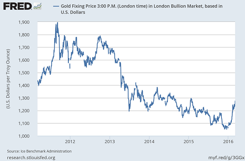
"Between September 2011's gold price high of over $1,900/ounce"(HERE).
- I considered two different distributions for the residuals (negatives and positives).
- I ran the arithmetic mean of both positive residuals and negative residuals (the statistically not significant residuals that are those that fall in the 95% area of the normal distribution).
By taking into consideration the findings of the before mentioned study on the historical volatility and my findings, I will keep an estimate for the historical gold price volatility (gamma) being± 25%.
The trend has changed its slope over time, it has become more steeply with respect to the axis of t. The driving force exerted by the Chinese demand that reached its record level in 2013 when the country became the world's largest gold market, leads me to keep an average historical volatility at ±25% around the gold price trend line.
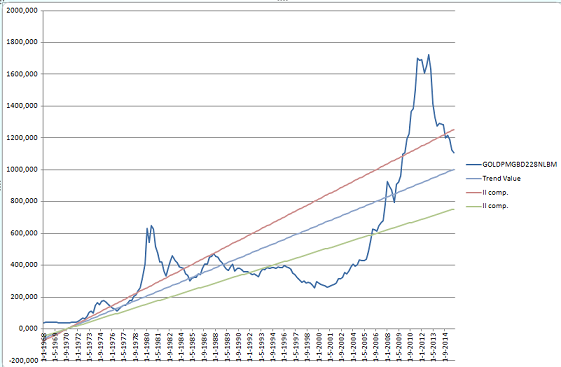
The mathematical equation of the gold price till the 2nd component is:
Yt (Gold price) = 471,227 + 5,57 x t' + 5,57 x ( 1 ± 25%) + 3rd component + error.
Fig. 2. The quarterly historical trend of nominal gold price, first component (drift) and second component from January 1968 to December 2015.
Third component (measurement of the seasonal variations with dummy variables):
I use a different approach to estimate the 3rd component (the jump and dip component) from the one used by the authors, but still based on dummy variables:
D1: D1 = 1 gold price had a jump otherwise, D1 = 0, gold price didn't have a jump.
D2:D2 = 1 gold price had a dip, otherwise, D2 = 0, gold price didn't have a dip.
I have a suspicion that jumps (D1:D1=1) and dips (D2:D2 =1) might be dependent, and hence not really are adding two separate variables to the multiple regression model to measure the effects on the gold price of jumps and dips, the predictor (independent) variables (the price of gold is the dependent variable). Essentially, this follows the model:
Yt = Alfa + Beta0 * t + Beta1* D1 + Beta2* D2 + error
I ran a simple linear regression analysis on both variables separately:
| SUMMARY OUTPUT | | | | | | |
| | | | | | | |
| Regression Statistics | | | | | |
| Multiple R | 0,769239473 | | | | | |
| R Square | 0,591729368 | | | | | |
| Adjusted R Square | 0,587386063 | | | | | |
| Standard Error | 257,9117581 | | | | | |
| Observations | 191 | | | | | |
| | | | | | | |
| ANOVA | | | | | | |
| | df | SS | MS | F | Significance F | |
| Regression | 2 | 18124879 | 9062439 | 136,2394 | 2,68612E-37 | |
| Residual | 188 | 12505473 | 66518,47 | | | |
| Total | 190 | 30630352 | | | | |
| | | | | | | |
| | Coefficients | Standard Error | t Stat | P-value | Lower 95% | Upper 95% |
| Intercept | 459,1438532 | 27,36744 | 16,77701 | 3,26E-39 | 405,157121 | 513,1306 |
| Time (NYSE:T) | 5,591915342 | 0,338825 | 16,50386 | 2,06E-38 | 4,923528366 | 6,260302 |
| D1 | 16,42982552 | 37,44986 | 0,438715 | 0,661372 | -57,44611934 | 90,30577 |
| SUMMARY OUTPUT | | | | | | |
| | | | | | | |
| Regression Statistics | | | | | |
| Multiple R | 0,769239473 | | | | | |
| R Square | 0,591729368 | | | | | |
| Adjusted R Square | 0,587386063 | | | | | |
| Standard Error | 257,9117581 | | | | | |
| Observations | 191 | | | | | |
| | | | | | | |
| ANOVA | | | | | | |
| | df | SS | MS | F | Significance F | |
| Regression | 2 | 18124878,98 | 9062439 | 136,2394 | 2,68612E-37 | |
| Residual | 188 | 12505473,3 | 66518,47 | | | |
| Total | 190 | 30630352,28 | | | | |
| | | | | | | |
| | Coefficients | Standard Error | t Stat | P-value | Lower 95% | Upper 95% |
| Intercept | 475,5736787 | 25,54124327 | 18,61983 | 1,53E-44 | 425,1894221 | 525,9579 |
| Time | 5,591915342 | 0,338824774 | 16,50386 | 2,06E-38 | 4,923528366 | 6,260302 |
| D2 | -16,42982552 | 37,44986245 | -0,43872 | 0,661372 | -90,30577039 | 57,44612 |
A jump (D1: D1=1) is on average $16.43 per troy ounce of gold over the period January 1968 - December 2015.
The quarterly average price of gold is $459.144; the quarterly price of gold per troy ounce is higher by $16.43 than the average quarterly price for a jump. Let's say about 3.58% (on average).
A dip (D2: D2=1) is on average -$16.43 per troy ounce of gold over the period January 1968 - December 2015.
The quarterly average price of gold is $475.574; the quarterly price of gold per troy ounce is lower by $16.43 than the average quarterly price for a dip. Let's say about -3.45% (on average).
The error approximates the existence of other components and the historical volatility.
The problem is that both parameters for D1 and D2 are not statistically significant at 5% level of confidence.
So I ran a regression on the price of gold over the observed period. Then I have calculated the average of jumps (positive returns) and dips (negative returns) of the statistically significant residuals at a 5% level of confidence.
Therefore the statistically significant jumps and dips are:
D1: D1=1, jump: +5.74%,
D2:D2=1, dip: -3.62%.
Conclusion:
"The proposed model was validated with historical gold prices. The model was then applied to forecast the gold price for the next 10 years. The results indicated that, assuming the current price jump initiated in 2007 behaves in the same manner as that experienced in 1978, the gold price would stay abnormally high up to the end of 2014. After that, the price would revert to the long-term trend until 2018."(here).
I made some variations to the proposed model of the mentioned study.
The average quarterly price of gold stayed abnormally high up to the first quarter of 2013, $1,631.774 per troy ounce, and then it started its descending phase. The average quarterly price of gold was $1,106.451 per troy ounce in the 4th quarter of 2015. It fell by 32% in 3 years.
The table below shows my forecast of average quarterly price of gold with statistically and not statistically significant jumps and dips until 2018:

The findings of the before mentioned study and my analysis on the time series of gold price lead me to conclude that 2016 will not be the right year for a substantial increase in gold price as I have several times written in my previous articles on gold mining stocks on NYSE:ABX, NYSE:GG and NYSE:NEM (read here, here and here).